How to Track Your Brand in AI Search

Traditional SEO reporting used to be simple: you tracked rankings, checked impressions and clicks in Search Console, and mapped those numbers to business impact. AI-driven search has reshaped that flow. Platforms like Google AI Overviews, AI Mode, Perplexity, and Bing Copilot no longer just list results – they generate answers and choose which sources to reference. That shift means the key question is no longer “do we rank?” but “are we being cited in the generative layer?”

The challenge is that this answer layer doesn’t sit neatly inside existing analytics tools, and it isn’t stable. A query that cites your brand today might not include you tomorrow, even if nothing on your site changed. GEO analytics is about shining light on this hidden layer, tracking how it moves, and connecting those appearances to measurable results.

Active vs Passive Ways to Spot Visibility

A reliable GEO measurement setup blends two approaches: actively checking where you show up and passively watching how search systems interact with your site.

Active detection means building your own monitoring agents that query AI search engines, capture the responses, and check for mentions of your domain. This could be as lightweight as a browser automation script that runs a set of queries and saves screenshots, or as advanced as a full pipeline that stores structured citation data from HTML or JSON outputs. The important part is repetition — AI answers are regenerated each time, so you need to run these agents often to capture how results shift. That variation is useful data in itself, especially when you compare it against changes in your own content or the wider competitive set.

Passive detection comes from your server logs. By tracking requests from AI crawlers, you can see when these systems fetch your pages. For example, if you notice PerplexityBot hitting certain URLs more frequently and then spot an uptick in citations for those same pages, you’ve uncovered a clear connection between retrieval and exposure. With more advanced parsing, you can group these bot visits by page and understand which parts of your site are being prioritized.

Tracking AI Search Bots

One of the most direct ways to understand how your content feeds into generative answers is to keep a close eye on the bots that crawl your site. These user agents represent the retrieval layer for platforms such as ChatGPT, Claude, Perplexity, Bing Copilot, and others. By monitoring them in your server logs, you get an early signal of when and how your content is being collected for potential inclusion in AI-generated responses.

This visibility matters because changes in crawl activity often align with shifts in your presence across AI search features. If certain bots increase their visits, it can indicate a stronger chance of your pages being retrieved and cited. Building and maintaining an up-to-date list of these crawlers, then matching their activity to your generative visibility, gives you one of the few tangible ways to measure a process that otherwise operates in the dark.

Vendor	User Agent / Token	Purpose	How to Manage	Extra Notes
OpenAI	GPTBot	Collects content for OpenAI model training	Block or allow in robots.txt (User-agent: GPTBot)	Documented on OpenAI’s official site
	OAI-SearchBot	Fetches pages for ChatGPT’s search results, not for training	User-agent: OAI-SearchBot	Used specifically for retrieval
Anthropic	ClaudeBot	Broad crawler for Claude model training	Control with robots.txt	Publicly explained in Anthropic’s help docs
	Claude-User	Fetcher triggered during live user queries	User-agent: Claude-User	Distinct from training bot
Perplexity	PerplexityBot	Main crawler that builds Perplexity’s index	User-agent: PerplexityBot	Publishes IP ranges and bot details
	Perplexity-User	Request-time fetcher when a user asks a question	User-agent: Perplexity-User	Not used for long-term indexing
Google	Googlebot Family	Standard crawlers for web, images, video, etc.	Controlled in robots.txt	Feeds both Search and generative features
	Google-Extended	Token that governs use of your content in AI features	Add in robots.txt as User-agent: Google-Extended	Not a crawler itself, just a control switch
Microsoft	bingbot	Bing’s primary crawler, also used for Copilot	User-agent: bingbot	Behaves like Googlebot with AI integration
Apple	Applebot	Crawler for Siri, Spotlight, and Apple services	User-agent: Applebot	Standard Apple crawler
	Applebot-Extended	Token for opting out of Apple’s AI training use	Control in robots.txt	Only affects model training, not crawling

Shaping Visibility With NUOPTIMA

At NUOPTIMA, we see visibility as more than search rankings. In AI-driven results, the question is whether your brand is recognized, cited, and trusted in the answer itself. That’s why we align classic SEO with Generative Engine Optimization – helping brands earn presence where it matters most.

We combine strategy, data, and execution to make sure your content is both retrievable by AI systems and impactful for real users. Our work spans technical SEO, international optimization, and content built to drive measurable growth. The result is stronger visibility that translates directly into business outcomes.

Why Brands Choose Us:

• Proven results with 70+ industry leaders across multiple sectors
• 3x average return on ad spend across organic and paid campaigns
• Expertise in scaling SaaS, eCommerce, healthcare, and more
• A balance of AI-driven insights with human-led strategy

Our approach isn’t about chasing vanity metrics. It’s about building visibility that sticks — presence in AI answers, credibility with users, and lasting gains in traffic and revenue. By focusing on how AI systems retrieve and cite information, we help brands secure a position in the conversations that drive decisions.

We also understand that every business is different. That’s why we tailor strategies to match your industry, your audience, and your growth goals. Whether you’re a startup looking for traction or an established company scaling globally, we apply the same data-driven mindset to deliver results you can measure.

At the end of the day, our mission is simple: make sure your brand doesn’t just appear in search, but that it stands out in the AI-powered future of discovery.

Detecting AI Overviews and AI Mode

Google runs both AI Overviews and AI Mode on top of its generative systems, but the two behave differently, which means you need separate ways of measuring them.

AI Overviews

Overviews appear directly within the search results page, usually when Google decides a quick, synthesized summary will improve the experience. Spotting them requires more than glancing at rankings. You need to capture the full SERP, scan for the Overview block, and check whether your site is being referenced in the answer or linked as a source.

The challenge is that Overviews aren’t fixed. A query might trigger one result in the morning and a completely different set in the afternoon. Sometimes the block disappears altogether. That instability makes ongoing tracking essential – one screenshot tells you almost nothing, but repeated checks reveal the real pattern of your presence.

AI Mode

AI Mode works differently. It sits in its own tab and produces longer, conversational responses. Because it aims to sustain a dialogue, the sources it cites often diverge from those shown in Overviews. Measuring visibility here means capturing the full conversation output and extracting every link included.

By comparing the two: Overviews and AI Mode – you can see how Google favors different sites depending on context. This side-by-side view often uncovers platform biases and shows where your brand is strong in one environment but missing in the other.

Tracking AI Overviews and AI Mode With FetchSERP

One of the simplest ways to monitor your visibility in Google’s AI surfaces is through FetchSERP. The platform provides a set of API endpoints that can return both traditional SERP data and generative results. For GEO tracking, the two endpoints that matter most are:

• /serp_ai – combines AI Overview and AI Mode in one payload whenever they’re available.
• /serp_ai_mode – a faster, US-only endpoint that focuses specifically on AI Mode results.

Both require an API token in the header, and each request needs your search query plus an optional country parameter (default is US).

How It Maps Into Sheets

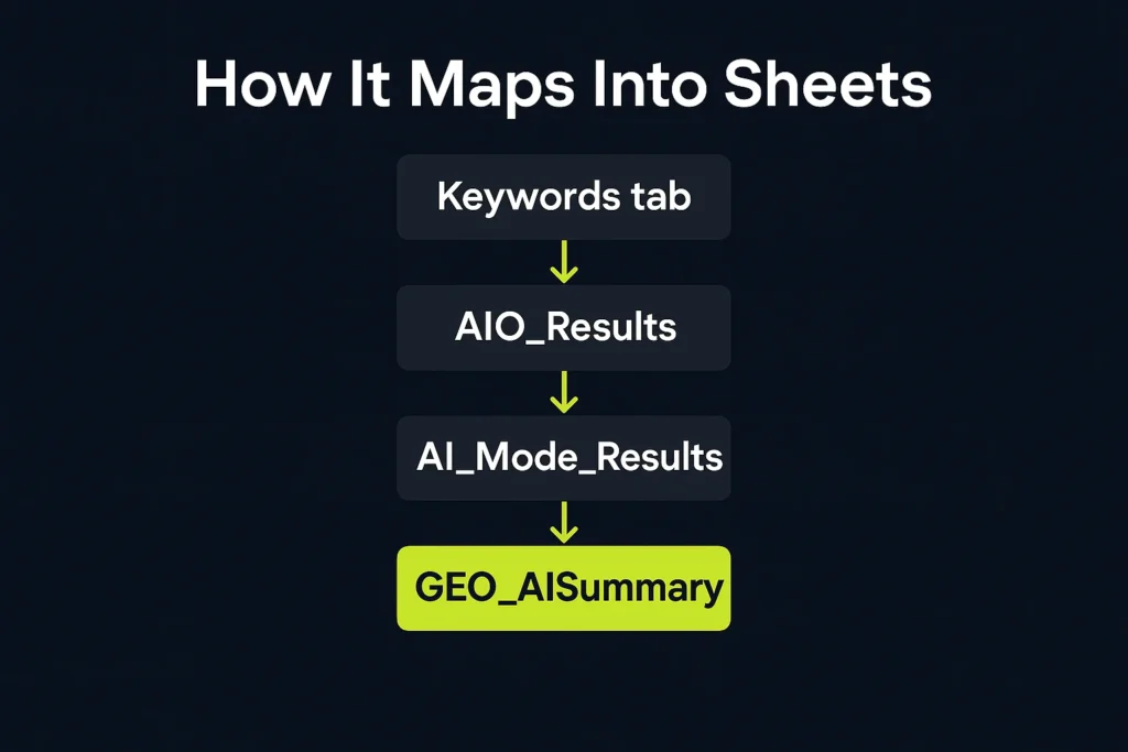
To keep everything organized, you’ll want to connect these API calls to a Google Sheet. Here’s the structure that works best:

• Keywords tab: Your query list (column A should be “keyword,” followed by one query per row).
• AIO_Results: Automatically populated with flags and source details whenever an AI Overview shows your brand.
• AI_Mode_Results: Similar output for AI Mode queries.
• GEO_AISummary: A running summary with charts that show how many queries triggered each AI surface.

Every time the script runs, it appends new rows with a timestamp. This means you can build a historical log that shows not just if you’re cited, but how that visibility changes over time.

Why This Matters

Running the script multiple times per day helps you capture short-term swings, while daily runs build a reliable long-term view. Over time, you can:

• Track frequency and consistency of citations
• Compare citation order and positioning
• Spot patterns in volatility versus stability

Setting Up the Script

In Google Sheets, you’ll add the script through Extensions → Apps Script. Before the first run, set your API key under Project Settings with the property name FETCHSERP_API_TOKEN. Once saved, paste in the script, reload the Sheet, and you’ll see a new menu option: GEO (FetchSERP) → Fetch AIO & AI Mode.

/**

 * FetchSERP → Google Sheets tracker for AI Overviews (AIO) and AI Mode

 * with rank-like signals and brand presence pivot.

 *

 * Tabs expected/created:

 *  – Keywords: column A header “keyword”, then one query per row.

 *  – Brands: column A header “domain” (your brand domains, no www).

 *  – AIO_Results: appended per run (presence + top domains).

 *  – AI_Mode_Results: appended per run (presence + top domains).

 *  – AI_Sources: appended per run (1 row per citation with rank and metadata).

 *  – GEO_AISummary: summary counts + chart (AIO vs AI Mode triggers).

 *  – GEO_BrandPresence: pivot for latest run + chart of rank-1 shares.

 */

const FETCHSERP_BASE = ‘https://www.fetchserp.com/api/v1’;

const DEFAULT_COUNTRY = ‘us’;

function onOpen() {

  SpreadsheetApp.getUi()

    .createMenu(‘GEO (FetchSERP)’)

    .addItem(‘Fetch AIO & AI Mode’, ‘runAIOTracking’)

    .addToUi();

}

function runAIOTracking() {

  const ss = SpreadsheetApp.getActiveSpreadsheet();

  const token = getApiToken_();

  const keywords = getKeywords_(ss);

  ensureBrandsSheet_(ss); // make sure Brands exists (empty is fine)

  const aioSheet = ensureSheet_(ss, ‘AIO_Results’, [

    ‘timestamp’, ‘keyword’, ‘country’,

    ‘has_ai_overview’, ‘source_count’, ‘top_source_domain’, ‘all_sources’

  ]);

  const aimodeSheet = ensureSheet_(ss, ‘AI_Mode_Results’, [

    ‘timestamp’, ‘keyword’, ‘country’,

    ‘has_ai_mode’, ‘source_count’, ‘top_source_domain’, ‘all_sources’

  ]);

  const srcSheet = ensureSheet_(ss, ‘AI_Sources’, [

    ‘timestamp’, ‘keyword’, ‘country’, ‘surface’, // AIO or AI_MODE

    ‘rank’, ‘url’, ‘domain’, ‘title’, ‘site_name’

  ]);

  const now = new Date();

  const aioRows = [];

  const aimodeRows = [];

  const sourceRows = [];

  for (const kw of keywords) {

    const country = DEFAULT_COUNTRY;

    // Primary combined endpoint

    const aiData = callFetchSerp_(‘serp_ai’, { query: kw, country }, token);

    // Optional AI Mode accelerator (US-only, cached)

    let aiModeData = null;

    try {

      aiModeData = callFetchSerp_(‘serp_ai_mode’, { query: kw }, token);

    } catch (e) {

      // OK to ignore; not always necessary

    }

    // —- AI OVERVIEW —-

    const aioBlock = getBlock_(aiData, ‘ai_overview’);

    const aioSources = normalizeSources_(aioBlock && aioBlock.sources);

    const aioTop = aioSources.length ? aioSources[0] : null;

    aioRows.push([

      now, kw, country,

      !!aioBlock,

      aioSources.length,

      aioTop ? domainOnly_(aioTop.url || aioTop.site_name || ”) : ”,

      aioSources.map(s => domainOnly_(s.url || s.site_name || ”)).join(‘ | ‘)

    ]);

    // push detailed sources with rank

    aioSources.forEach((s, i) => {

      sourceRows.push([

        now, kw, country, ‘AIO’,

        i + 1,

        s.url || ”,

        domainOnly_(s.url || s.site_name || ”),

        s.title || ”,

        s.site_name || ”

      ]);

    });

    // —- AI MODE —-

    const aiModeBlock = extractAiMode_(aiModeData) || extractAiMode_(aiData);

    const aimSources = normalizeSources_(aiModeBlock && aiModeBlock.sources);

    const aimTop = aimSources.length ? aimSources[0] : null;

    aimodeRows.push([

      now, kw, country,

      !!aiModeBlock,

      aimSources.length,

      aimTop ? domainOnly_(aimTop.url || aimTop.site_name || ”) : ”,

      aimSources.map(s => domainOnly_(s.url || s.site_name || ”)).join(‘ | ‘)

    ]);

    aimSources.forEach((s, i) => {

      sourceRows.push([

        now, kw, country, ‘AI_MODE’,

        i + 1,

        s.url || ”,

        domainOnly_(s.url || s.site_name || ”),

        s.title || ”,

        s.site_name || ”

      ]);

    });

    Utilities.sleep(400); // rate-friendly

  }

  if (aioRows.length) appendRows_(aioSheet, aioRows);

  if (aimodeRows.length) appendRows_(aimodeSheet, aimodeRows);

  if (sourceRows.length) appendRows_(srcSheet, sourceRows);

  buildSummaryAndChart_();

  buildBrandPresencePivotAndChart_(); // NEW

}

/* ———————– Helpers & Builders ———————– */

function getApiToken_() {

  const props = PropertiesService.getScriptProperties();

  const token = props.getProperty(‘FETCHSERP_API_TOKEN’) || ”;

  if (!token) {

    throw new Error(‘Missing FETCHSERP_API_TOKEN in Script properties. Set it in Project Settings.’);

  }

  return token;

}

function getKeywords_(ss) {

  const sh = ss.getSheetByName(‘Keywords’);

  if (!sh) throw new Error(‘Missing “Keywords” sheet with header “keyword” in A1.’);

  const values = sh.getRange(2, 1, Math.max(0, sh.getLastRow() – 1), 1)

    .getValues().flat().map(String).map(s => s.trim()).filter(Boolean);

  if (!values.length) throw new Error(‘No keywords found under header “keyword” (A2:A).’);

  return values;

}

function ensureSheet_(ss, name, headers) {

  let sh = ss.getSheetByName(name);

  if (!sh) sh = ss.insertSheet(name);

  if (sh.getLastRow() === 0) {

    sh.getRange(1, 1, 1, headers.length).setValues([headers]);

    sh.setFrozenRows(1);

  }

  return sh;

}

function ensureBrandsSheet_(ss) {

  let sh = ss.getSheetByName(‘Brands’);

  if (!sh) {

    sh = ss.insertSheet(‘Brands’);

    sh.getRange(1, 1).setValue(‘domain’);

    sh.setFrozenRows(1);

  }

  return sh;

}

function callFetchSerp_(path, params, token) {

  const url = `${FETCHSERP_BASE}/${path}?` + Object.keys(params)

    .map(k => `${encodeURIComponent(k)}=${encodeURIComponent(params[k])}`).join(‘&’);

  const res = UrlFetchApp.fetch(url, {

    method: ‘get’,

    headers: { ‘accept’: ‘application/json’, ‘authorization’: `Bearer ${token}` },

    muteHttpExceptions: true

  });

  const code = res.getResponseCode();

  const text = res.getContentText();

  if (code < 200 || code >= 300) throw new Error(`FetchSERP ${path} error ${code}: ${text}`);

  try { return JSON.parse(text); }

  catch (e) { throw new Error(`FetchSERP ${path} invalid JSON: ${text.slice(0, 300)}…`); }

}

function getBlock_(payload, key) {

  if (!payload) return null;

  const d = payload.data || payload;

  if (d.results && d.results[key]) return d.results[key];

  if (d[key]) return d[key];

  return null;

}

function extractAiMode_(payload) { // tolerate different shapes

  if (!payload) return null;

  const d = payload.data || payload;

  if (d.results && d.results.ai_mode) return d.results.ai_mode;

  if (d.ai_mode) return d.ai_mode;

  return null;

}

function normalizeSources_(sources) {

  if (!Array.isArray(sources)) return [];

  return sources

    .map(s => s || Array)

    .map(s => ({

      url: s.url || ”,

      title: s.title || ”,

      site_name: s.site_name || ”

    }))

    .filter(s => s.url || s.site_name);

}

function domainOnly_(u) {

  try {

    const host = (new URL(u)).hostname || ”;

    return host.replace(/^www\./i, ”);

  } catch (e) {

    return (u || ”).replace(/^www\./i, ”);

  }

}

function appendRows_(sheet, rows) {

  sheet.getRange(sheet.getLastRow() + 1, 1, rows.length, rows[0].length).setValues(rows);

}

/** Create or refresh a historical summary tab with counts & share of voice, plus trend chart. */

/** Create or refresh a historical summary tab with counts, SOV, and 7-day rolling averages, plus a trend chart. */

function buildSummaryAndChart_() {

  const ss = SpreadsheetApp.getActiveSpreadsheet();

  const sum = ensureSheet_(ss, ‘GEO_AISummary’, [

    ‘date’,

    ‘AIO_count’, ‘AIO_share_of_voice’,

    ‘AI_Mode_count’, ‘AI_Mode_share_of_voice’,

    ‘keywords_tracked’,

    ‘AIO_count_7dma’, ‘AI_Mode_count_7dma’,

    ‘AIO_sov_7dma’, ‘AI_Mode_sov_7dma’

  ]);

  // Clear old rows (keep header)

  if (sum.getLastRow() > 1) {

    sum.getRange(2, 1, sum.getLastRow() – 1, 11).clearContent();

  }

  const aio = ss.getSheetByName(‘AIO_Results’);

  const aim = ss.getSheetByName(‘AI_Mode_Results’);

  const kwSheet = ss.getSheetByName(‘Keywords’);

  if (!aio || !aim || !kwSheet) return;

  const keywordsTracked = Math.max(0, kwSheet.getLastRow() – 1);

  // Build daily counts maps

  const aioCounts = countByDate_(aio, 1, 4); // timestamp col 1, has_ai_overview col 4

  const aimCounts = countByDate_(aim, 1, 4); // timestamp col 1, has_ai_mode col 4

  const allDates = Array.from(new Set([…Object.keys(aioCounts), …Object.keys(aimCounts)]))

    .sort((a, b) => new Date(a) – new Date(b));

  // Build rows with daily values first

  const rows = allDates.map(date => {

    const aCount = aioCounts[date] || 0;

    const mCount = aimCounts[date] || 0;

    const aSOV = keywordsTracked ? aCount / keywordsTracked : 0;

    const mSOV = keywordsTracked ? mCount / keywordsTracked : 0;

    return [

      date,

      aCount, aSOV,

      mCount, mSOV,

      keywordsTracked,

      null, null, // AIO_count_7dma, AI_Mode_count_7dma (fill after)

      null, null  // AIO_sov_7dma, AI_Mode_sov_7dma (fill after)

    ];

  });

  // Compute 7-day rolling averages (centered on the last 7 days ending at index i)

  const aCountSeries = rows.map(r => r[1]);

  const mCountSeries = rows.map(r => r[3]);

  const aSovSeries   = rows.map(r => r[2]);

  const mSovSeries   = rows.map(r => r[4]);

  const aCount7 = rollingMean_(aCountSeries, 7);

  const mCount7 = rollingMean_(mCountSeries, 7);

  const aSov7   = rollingMean_(aSovSeries,   7);

  const mSov7   = rollingMean_(mSovSeries,   7);

  // Fill the rolling columns

  for (let i = 0; i < rows.length; i++) {

    rows[i][6]  = aCount7[i]; // AIO_count_7dma

    rows[i][7]  = mCount7[i]; // AI_Mode_count_7dma

    rows[i][8]  = aSov7[i];   // AIO_sov_7dma

    rows[i][9]  = mSov7[i];   // AI_Mode_sov_7dma

  }

  if (rows.length) {

    sum.getRange(2, 1, rows.length, rows[0].length).setValues(rows);

  }

  // Rebuild chart: daily counts + smoothed SOV on dual axes

  const charts = sum.getCharts();

  charts.forEach(c => sum.removeChart(c));

  const dataHeight = rows.length + 1; // include header

  const chart = sum.newChart()

    .setChartType(Charts.ChartType.LINE)

    .addRange(sum.getRange(1, 1, dataHeight, 10)) // includes counts, SOV, and 7d SOV

    .setPosition(5, 1, 0, 0)

    .setOption(‘title’, ‘AIO & AI Mode — Daily Counts and 7-Day SOV Averages’)

    .setOption(‘hAxis’, { title: ‘Date’ })

    .setOption(‘vAxes’, {

      0: { title: ‘Keyword Count’ },

      1: { title: ‘Share of Voice (7-day avg)’, format: ‘percent’ }

    })

    // Series mapping: 0=AIO_count, 1=AIO_SOV, 2=AI_Mode_count, 3=AI_Mode_SOV, 4=keywords_tracked,

    //                 5=AIO_count_7dma, 6=AI_Mode_count_7dma, 7=AIO_sov_7dma, 8=AI_Mode_sov_7dma

    // We’ll show daily counts (0,2) on axis 0, hide raw daily SOV (1,3) to reduce noise,

    // show smoothed SOV (7,8) on axis 1, and hide keywords_tracked (4) + count_7dma (5,6) from display.

    .setOption(‘series’, {

      0: { targetAxisIndex: 0 }, // AIO_count (line)

      1: { targetAxisIndex: 1, visibleInLegend: false, lineWidth: 0, pointsVisible: false }, // raw AIO SOV (hidden)

      2: { targetAxisIndex: 0 }, // AI_Mode_count (line)

      3: { targetAxisIndex: 1, visibleInLegend: false, lineWidth: 0, pointsVisible: false }, // raw AI Mode SOV (hidden)

      4: { visibleInLegend: false, lineWidth: 0, pointsVisible: false }, // keywords_tracked (hidden)

      5: { visibleInLegend: false, lineWidth: 0, pointsVisible: false }, // AIO_count_7dma (hidden to avoid clutter)

      6: { visibleInLegend: false, lineWidth: 0, pointsVisible: false }, // AI_Mode_count_7dma (hidden)

      7: { targetAxisIndex: 1 }, // AIO_sov_7dma (smooth)

      8: { targetAxisIndex: 1 }  // AI_Mode_sov_7dma (smooth)

    })

    .setOption(‘legend’, { position: ‘bottom’ })

    .build();

  sum.insertChart(chart);

}

/** Simple trailing rolling mean with window W; returns array aligned to input length (nulls until window is filled). */

function rollingMean_(arr, W) {

  const out = new Array(arr.length).fill(null);

  let sum = 0;

  for (let i = 0; i < arr.length; i++) {

    sum += (typeof arr[i] === ‘number’ ? arr[i] : 0);

    if (i >= W) sum -= (typeof arr[i – W] === ‘number’ ? arr[i – W] : 0);

    if (i >= W – 1) out[i] = sum / W;

  }

  return out;

}

/** Helper: count how many rows have TRUE in booleanCol, grouped by date from dateCol. */

function countByDate_(sheet, dateCol, booleanCol) {

  const rows = sheet.getRange(2, 1, sheet.getLastRow() – 1, sheet.getLastColumn()).getValues();

  const counts = Array;

  rows.forEach(row => {

    const ts = row[dateCol – 1];

    const has = row[booleanCol – 1];

    if (ts && (has === true || has === ‘TRUE’)) {

      const d = new Date(ts);

      const dateStr = Utilities.formatDate(d, Session.getScriptTimeZone(), ‘yyyy-MM-dd’);

      counts[dateStr] = (counts[dateStr] || 0) + 1;

    }

  });

  return counts;

}

function countTrue_(sheet, col) {

  if (!sheet || sheet.getLastRow() < 2) return 0;

  const vals = sheet.getRange(2, col, sheet.getLastRow() – 1, 1).getValues().flat();

  return vals.filter(v => v === true || v === ‘TRUE’).length;

}

/**

 * Build a pivot for BRAND presence (latest run only).

 * For each surface (AIO / AI_MODE), we compute:

 *  – queries_with_surface: number of keywords where that surface triggered

 *  – queries_brand_cited: number of those keywords where brand domain appears in any citation

 *  – presence_rate = brand_cited / queries_with_surface

 *  – queries_brand_rank1: number where brand is rank 1 citation

 *  – rank1_rate = brand_rank1 / queries_with_surface

 */

function buildBrandPresencePivotAndChart_() {

  const ss = SpreadsheetApp.getActiveSpreadsheet();

  const brands = readBrands_(ss); // array of domains (no www)

  const aioSheet = ss.getSheetByName(‘AIO_Results’);

  const aimSheet = ss.getSheetByName(‘AI_Mode_Results’);

  const srcSheet = ss.getSheetByName(‘AI_Sources’);

  if (!brands.length || !srcSheet || srcSheet.getLastRow() < 2) {

    ensureSheet_(ss, ‘GEO_BrandPresence’, [‘brand_domain’, ‘surface’, ‘queries_with_surface’, ‘queries_brand_cited’, ‘presence_rate’, ‘queries_brand_rank1’, ‘rank1_rate’]);

    return;

  }

  // Determine latest run timestamp (max timestamp across results)

  const latest = latestTimestamp_([aioSheet, aimSheet, srcSheet].filter(Boolean));

  if (!latest) return;

  // Build per-surface sets of keywords that triggered surface in the latest run

  const latestAioKeywords = new Set(filterKeywordsByTimestampAndBool_(aioSheet, latest, 4)); // has_ai_overview

  const latestAimKeywords = new Set(filterKeywordsByTimestampAndBool_(aimSheet, latest, 4)); // has_ai_mode

  // Build maps for brand presence by keyword and rank1 by keyword (latest run only)

  const surfaceBrandAny = { AIO: new Map(), AI_MODE: new Map() }; // brand -> Set(keywords)

  const surfaceBrandRank1 = { AIO: new Map(), AI_MODE: new Map() }; // brand -> Set(keywords)

  // Iterate source rows for latest timestamp only

  const srcVals = srcSheet.getRange(2, 1, srcSheet.getLastRow() – 1, 9).getValues();

  for (const row of srcVals) {

    const [ts, kw, country, surface, rank, url, domain/*clean*/, title, site_name] = row;

    if (!sameDay_(ts, latest)) continue; // group by day/run timestamp granularity

    const dom = String(domain || ”).toLowerCase();

    if (!dom) continue;

    // For presence calculations, only consider keywords that triggered that surface

    if (surface === ‘AIO’ && !latestAioKeywords.has(kw)) continue;

    if (surface === ‘AI_MODE’ && !latestAimKeywords.has(kw)) continue;

    // For each brand, check match

    for (const b of brands) {

      if (dom.endsWith(b)) {

        // any-cited

        if (!surfaceBrandAny[surface].has(b)) surfaceBrandAny[surface].set(b, new Set());

        surfaceBrandAny[surface].get(b).add(kw);

        // rank1

        if (rank === 1) {

          if (!surfaceBrandRank1[surface].has(b)) surfaceBrandRank1[surface].set(b, new Set());

          surfaceBrandRank1[surface].get(b).add(kw);

        }

      }

    }

  }

  // Prepare output rows

  const out = [];

  const surfaces = [‘AIO’, ‘AI_MODE’];

  for (const s of surfaces) {

    const queriesWithSurface = (s === ‘AIO’) ? latestAioKeywords.size : latestAimKeywords.size;

    for (const b of brands) {

      const cited = surfaceBrandAny[s].get(b)?.size || 0;

      const r1 = surfaceBrandRank1[s].get(b)?.size || 0;

      const presenceRate = queriesWithSurface ? (cited / queriesWithSurface) : 0;

      const rank1Rate = queriesWithSurface ? (r1 / queriesWithSurface) : 0;

      out.push([

        b, s, queriesWithSurface, cited, presenceRate, r1, rank1Rate

      ]);

    }

  }

  const pivot = ensureSheet_(ss, ‘GEO_BrandPresence’, [‘brand_domain’, ‘surface’, ‘queries_with_surface’, ‘queries_brand_cited’, ‘presence_rate’, ‘queries_brand_rank1’, ‘rank1_rate’]);

  // Clear old data

  if (pivot.getLastRow() > 1) pivot.getRange(2, 1, pivot.getLastRow() – 1, 7).clearContent();

  if (out.length) pivot.getRange(2, 1, out.length, 7).setValues(out);

  // Build/refresh a chart for Rank-1 share per brand per surface

  const charts = pivot.getCharts();

  charts.forEach(c => pivot.removeChart(c));

  // Simple approach: chart all rows, data has both surfaces; users can filter in Sheets UI.

  const chart = pivot.newChart()

    .setChartType(Charts.ChartType.COLUMN)

    .addRange(pivot.getRange(1, 1, Math.max(2, pivot.getLastRow()), 7))

    .setPosition(5, 1, 0, 0)

    .setOption(‘title’, ‘Brand Rank-1 Share (latest run)’)

    .setOption(‘series’, {

      0: { targetAxisIndex: 0 }, // presence metrics

      1: { targetAxisIndex: 0 },

      2: { targetAxisIndex: 1 }  // rate on secondary axis if desired

    })

    .setOption(‘legend’, { position: ‘right’ })

    .build();

  pivot.insertChart(chart);

}

/* ———- Pivot helpers ———- */

function readBrands_(ss) {

  const sh = ss.getSheetByName(‘Brands’);

  if (!sh || sh.getLastRow() < 2) return [];

  const vals = sh.getRange(2, 1, sh.getLastRow() – 1, 1).getValues().flat()

    .map(String).map(v => v.trim().toLowerCase().replace(/^www\./, ”))

    .filter(Boolean);

  return Array.from(new Set(vals));

}

function latestTimestamp_(sheets) {

  let latest = null;

  for (const sh of sheets) {

    if (!sh || sh.getLastRow() < 2) continue;

    const tsCol = 1; // first col in our schemas

    const vals = sh.getRange(2, tsCol, sh.getLastRow() – 1, 1).getValues().flat();

    for (const v of vals) {

      const d = (v instanceof Date) ? v : new Date(v);

      if (!isNaN(+d)) {

        if (!latest || d > latest) latest = d;

      }

    }

  }

  return latest;

}

function sameDay_(a, b) {

  if (!(a instanceof Date)) a = new Date(a);

  if (!(b instanceof Date)) b = new Date(b);

  return a.getFullYear() === b.getFullYear() &&

         a.getMonth() === b.getMonth() &&

         a.getDate() === b.getDate();

}

function filterKeywordsByTimestampAndBool_(sheet, latestTs, boolColIndex) {

  if (!sheet || sheet.getLastRow() < 2) return [];

  const rows = sheet.getRange(2, 1, sheet.getLastRow() – 1, sheet.getLastColumn()).getValues();

  const out = [];

  for (const r of rows) {

    const ts = r[0];

    const kw = r[1];

    const val = r[boolColIndex – 1];

    if (sameDay_(ts, latestTs) && (val === true || val === ‘TRUE’)) out.push(kw);

  }

  return out;

}

From there, each run queries your keyword list, calls the endpoints, normalizes the output, and adds timestamped results into the proper tabs. Over time, this becomes a full dataset you can pivot, chart, and analyze – essentially a visibility dashboard you can control.

How FetchSERP Fits Into the Workflow

The script starts by calling /api/v1/serp_ai, which provides a combined snapshot of AI Overview and AI Mode results whenever they’re present. If you’re running queries from the US, the script also checks /api/v1/serp_ai_mode, a cached endpoint that delivers AI Mode data faster. When both are available, the cached AI Mode is preferred.

Inside the payload, you’ll usually find:

• AI Overview results stored under data.results.ai_overview
• AI Mode results under data.results.ai_mode

Each comes with an array of sources, which are then parsed into a clean list of domains. Those domains are what you’ll eventually use for pivoting and visibility charts.

Writing Results Into Sheets

The Google Apps Script connects directly to Sheets in a straightforward way:

• It checks that the Keywords tab is set up properly.
• If missing, it automatically creates the AIO_Results and AI_Mode_Results tabs.
• For every query run, it appends a new row that includes the timestamp, presence flags, number of sources, the top cited domain, and a list of all domains in that answer set.

Because new rows are added instead of overwritten, you gradually build a historical record. Over time, you can chart metrics like:

• The percentage of your tracked keywords that trigger an AI Overview
• The most frequently cited domains in AI Mode by week or month

This historical view is what turns one-off checks into actionable insights.

Best Practices for Using FetchSERP

1. Plan for volatility: AI answers are not fixed. Repeated sampling and timestamps are the only way to make sense of changes.
2. Avoid hitting limits: If you’re tracking large keyword sets, add pauses (e.g., Utilities.sleep(400)) or split them into batches.
3. Stay region-specific: Always pass a country code for queries, otherwise your data will mix locations.
4. Capture more detail: If you want deeper analysis, extend the script to also store full URLs, page titles, and publisher names.

While enterprise SaaS tools can give you polished dashboards, building your own pipeline with FetchSERP gives you flexibility and control. For many teams, it’s the quickest way to start treating AI visibility as a measurable, repeatable process.

How to Monitor Perplexity and Copilot

Perplexity

Perplexity is one of the easier platforms to measure because it displays its citations directly alongside the answer. Detection tools can grab those references as soon as they render. The catch is that Perplexity rarely sticks to the query you type. It quietly reformulates the question before pulling in results, which means part of the diagnostic process is capturing those reformulated queries. Without them, it’s hard to know why your content did or didn’t make the cut.

If you’re scraping Perplexity for tracking, these regions are most reliable:

• Answer text: usually appears in main [data-testid=”answer”], main article, or main .prose. As a fallback, look for classes containing prose or markdown.
• Citations list: often found in aside [data-testid=”source”] or nav[aria-label*=”Sources”] a[href]. Inline citations may appear as sup a[href] or a[data-source-id] inside the answer itself.
• Bonus method: Perplexity sometimes embeds a JSON state in script[type=”application/json”] or via a window.__… hydration object. Parsing this can give you a more stable list of sources – complete with titles, URLs, and authors, instead of relying only on the visible DOM.

Bing Copilot

Copilot introduces another set of challenges. It leans heavily on Bing’s index, so your baseline Bing visibility strongly affects whether you appear in its generative answers. Unlike Perplexity, Copilot tends to tuck citations at the end of its response, which reduces their visibility. Tracking requires capturing the entire AI block and parsing every link. By comparing Copilot’s citations against Bing’s standard rankings for the same query, you can identify whether rankings alone drive inclusion or if other authority signals are at play.

Turning AI Search Data Into a Dashboard

The end goal of all your monitoring is a single place where you can see how your brand performs across AI surfaces. A good dashboard pulls together both the active checks you run and the passive crawl data from your logs, then turns it into a clear view of where you stand.

What the Dashboard Should Show

Your dashboard shouldn’t just tell you if you’re cited – it should explain the context. For each keyword you track, you want to know:

• Did an AI Overview or AI Mode trigger?
• Was your content referenced, and how prominent was it?
• How often have you been cited in the last week or month?
• Do changes in bot crawl patterns line up with those citations?

With this setup, you can stop guessing about visibility and start spotting actual trends.

Key Metrics to Track

The most useful dashboards highlight:

• Daily Counts: Number of keywords that triggered AI Overviews or AI Mode.
• Share of Voice (SOV): Percentage of your keywords that show up in each feature.
• Rolling Averages: Seven-day trends that smooth out daily volatility and show the real trajectory.
• Brand Presence: Where your domain appears, and whether you’re cited first or buried down the list.

Turning Data Into Insight

By layering visibility data with server log activity, you can uncover which content updates, technical fixes, or competitive shifts are moving the needle. Over time, this cause-and-effect view helps you see not just whether you’re present in AI answers, but why. That’s the insight you need to guide your next round of optimizations.

Breakdown of GEO_AISummary Data

Column	Field	What It Shows
A	Date	The calendar date of the run, pulled from the timestamp
B	AIO_Count	Number of tracked keywords that triggered an AI Overview on that day
C	AIO_SOV	Share of voice for AI Overviews (AIO_Count ÷ total keywords)
D	AIMode_Count	Number of tracked keywords that triggered AI Mode
E	AIMode_SOV	Share of voice for AI Mode (AIMode_Count ÷ total keywords)
F	Keywords_Tracked	Total number of queries being monitored in your list
G	AIO_Count_7DayAvg	Seven-day rolling average of AI Overview counts
H	AIMode_Count_7DayAvg	Seven-day rolling average of AI Mode counts
I	AIO_SOV_7DayAvg	Seven-day rolling average of AI Overview share of voice
J	AIMode_SOV_7DayAvg	Seven-day rolling average of AI Mode share of voice

Setting Up a GEO Dashboard in Google Sheets

The script drops in a basic chart, but building your own dashboard inside Google Sheets gives you more control over how you view the data. With a few tweaks, you can turn a list of numbers into a clear picture of how your AI visibility is trending.

Step 1: Organize the Data

Open the GEO_AISummary tab. Make sure each column is labeled correctly, then sort by date from oldest to newest. This keeps the timeline straight before you start charting.

Step 2: Plot Daily Activity

Select columns A, B, and D (Date, AIO_Count, AIMode_Count). Insert a chart – a line or column chart works best here.

• X-axis: Date
• Series 1: AIO_Count
• Series 2: AIMode_Count

Give it a title such as ‘’Daily AI Overview and AI Mode Activity’’.

Step 3: Visualize Share of Voice

Highlight columns A, C, E, I, and J (Date, AIO_SOV, AIMode_SOV, plus the 7-day averages). Insert another line chart.

• Plot the raw daily percentages if you want to see short-term swings.
• Plot the rolling averages to reveal longer-term movement.

Label it something like ‘’Share of Voice Trends’’.

Step 4: Build the Dashboard View

Create a new sheet called ‘Dashboard’. Add both charts you just built, then create a small summary section at the top showing:

• Current counts and SOV for today
• Comparison to last week’s rolling average

Step 5: Track Over Time

Run the script each day (or more often if you need higher resolution). Because the data appends rather than overwrites, you’ll automatically create a running history. Over weeks and months, patterns will emerge – seasonal fluctuations, the impact of algorithm shifts, or the results of your optimization efforts.

Practical Tips for Reliable GEO Tracking

Working with AI search visibility is messy by nature. Systems are probabilistic, results shift constantly, and the same query can behave differently from one run to the next. These practices can help you get cleaner, more useful data.

Expect Volatility

Don’t assume stability. AI Overviews and AI Mode can change citations from one moment to the next. That’s why running checks regularly, and logging timestamps, is essential. The noise is part of the signal.

Manage Query Volume

If you’re monitoring hundreds of keywords, pace your requests. Add delays between runs or break large lists into smaller batches. This prevents hitting rate limits and keeps your data collection consistent.

Be Region-Specific

Always include a country code when running queries. Otherwise, your results might mix geographies, making it harder to interpret changes over time.

Track More Than Domains

Domains are a solid starting point, but sometimes you need deeper detail. Capture full URLs, page titles, and publisher names when it matters. This helps you see exactly which assets are earning visibility.

Keep Raw Data

AI platforms tweak their outputs often. Holding onto raw HTML or JSON responses means you can reprocess older data if parsers break or if you need to extract new fields later.

Conclusion

Generative search has rewritten the playbook for measuring visibility. Rankings and clicks alone no longer capture the full story – the real question is whether your brand is cited in the answers users actually see. By combining active detection with server log analysis, keeping tabs on AI crawlers, and building a dashboard that tracks both daily counts and long-term trends, you can turn an opaque system into measurable insights.

The work isn’t just about watching numbers climb. It’s about connecting those citations to real business outcomes: conversions, revenue, and growth. That’s what transforms visibility into value. With a consistent tracking framework in place, you’re no longer guessing about your presence in AI search. You’re making informed decisions that push your brand into the conversations that matter.

FAQ

1. Why is tracking AI search visibility so difficult?

Because AI answers regenerate each time, results can shift from one run to the next. Unlike traditional rankings, there’s no fixed position to rely on, which makes ongoing monitoring essential.

2. How often should I run tracking scripts?

For a small keyword set, multiple runs per day capture volatility. For larger lists, daily runs are usually enough to build a reliable trendline.

3. What’s the role of server logs in GEO analytics?

Server logs reveal when AI bots crawl your pages. Correlating crawl activity with citation data helps you understand how retrieval connects to visibility.

4. Do I need to track both AI Overviews and AI Mode?

Yes. They behave differently, and your brand might show up in one but not the other. Tracking both surfaces gives a complete picture of your Google AI presence.

5. Is Perplexity easier to measure than Google?

In some ways, yes. Perplexity shows citations transparently, but it also rewrites queries behind the scenes, so capturing reformulated questions is just as important as logging visible sources.